Analysis of a Rectangular Patch Antenna

This example uses the Hado high-frequency electromagnetic (EM) solver to calculate the frequency response of the input reflection coefficient ($S_{11}$) of a rectangular patch antenna [1,2].

The mesh required for the simulation is created using Gmsh in a separate Jupyter Notebook. The generated mesh is then imported into Hado, where material properties and boundary conditions are assigned before running the EM simulation.

Hado provides a Python-based workflow for importing meshes, assigning material properties and boundary conditions, performing finite element method (FEM) simulations, and visualizing the results.

The antenna’s reflection characteristics are evaluated in five steps:

1. Create the antenna geometry and generate the mesh using Gmsh.
2. Import the generated mesh into Hado.
3. Assign material properties and boundary conditions.
4. Run an EM simulation over a frequency sweep.
5. Plot the S-parameters.

Download Example Files

The ZIP file below contains the Jupyter Notebooks for mesh generation and electromagnetic simulation.

Download Example Files (ZIP)

After extracting the ZIP file, first run the mesh generation notebook to create patchAntenna.msh. Then run the electromagnetic simulation notebook to calculate the antenna’s reflection characteristics.

Import Libraries

Import the Python libraries needed for the simulation.

From Hado’s hado package, import the modules for boundary conditions, materials, high-frequency electromagnetic analysis, and meshes. NumPy is used to define the simulation frequencies.

from hado import boundary, material, highfrequency, mesh
import numpy as np

Define Parameters

Specify the frequency sweep, material properties, and dimensions of the lumped port.

freq = np.linspace(2.2e9,2.7e9,21)

epsilon_r_air = 1.0
loss_tangent_air = 0.0
epsilon_r_fr4 = 4.3
loss_tangent_fr4 = 0.015

port_width = 2.5e-3
port_height = 1.53e-3

Load Mesh

Load the mesh of the rectangular patch antenna.

This example uses a pre-generated mesh in Gmsh (.msh) format. The mesh defines volume regions for the dielectric substrate and surrounding air, as well as surfaces for the conductors and feed.

Hado uses domain IDs and boundary IDs defined in the mesh to assign material properties and boundary conditions, respectively.

em = highfrequency.HighFrequency()
em.mesh = mesh.Mesh("patchAntenna.msh")
em.mesh

Mesh
  filename          : patchAntenna.msh
  points            : [[ 0.00355     0.          0.        ]
 [ 0.00605     0.          0.        ]
 [ 0.00605     0.          0.00153   ]
 ...
 [-0.05865204 -0.02086738  0.02026195]
 [-0.00538913 -0.02339536  0.01281525]
 [ 0.01324966  0.01389609 -0.00275117]]
  elements          : [[ 105  581  582  922]
 [ 282  453  181  186]
 [ 350  496  404  950]
 ...
 [2113 2092  318 1491]
 [2092 2113  318  283]
 [ 283 2113  318  320]]
  boundary_elements : [[   2    3  333]
 [   3    2  345]
 [ 342  308    2]
 ...
 [1206 1157 1205]
 [1158 1162 1189]
 [1195 1192 1167]]
  domain            : [1 2]
  boundary          : [1 2 3]

Assign Materials and Boundary Conditions

Define the dielectric materials and boundary conditions used in the antenna model.

Material Properties

Assign FR-4 to the dielectric substrate and air to the surrounding region. For each material, specify the relative permittivity (epsilon_r) and dielectric loss tangent (loss_tangent).

Material	Relative permittivity	Dielectric loss tangent	Domain ID
FR4	4.3	0.015	1
Air	1.0	0.0	2

air = material.Dielectric(
    name="Air",
    epsilon_r=epsilon_r_air,
    loss_tangent=loss_tangent_air
)
fr4 = material.Dielectric(
    name="FR4",
    epsilon_r=epsilon_r_fr4,
    loss_tangent=loss_tangent_fr4
)
em.assign_material(fr4,domain=1)
em.assign_material(air,domain=2)

Boundary Conditions

This example uses three types of boundary conditions:

• Perfect electric conductor（PEC）：Models the top patch and bottom ground plane as ideal conductors with no conductor losses.
• Absorbing boundary condition（ABC）：Reduces artificial reflections of electromagnetic waves radiated from the antenna at the outer boundary of the computational domain.
• Lumped port：Excites the antenna at its feed and defines the excitation voltage and reference impedance.

The lumped port is configured with an excitation voltage of 1 V and a reference impedance of 50 Ω. Its dimensions, voltage direction, and power flow direction are also specified.

abc = boundary.Absorbing(2)
pec = boundary.PEC(1)
port = boundary.LumpedPort(3)
port.width = port_width
port.height = port_height
port.voltage_direction = [0.0, 0.0, 1.0]
port.power_flow_direction = "-y"
port.voltage = 1.0
port.impedance = complex(50.0, 0.0)
em.boundary = [abc, pec, port]

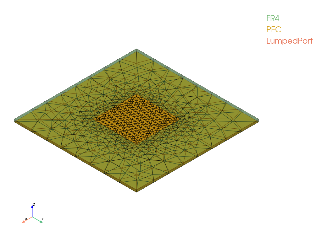
Use em.show() to visualize the antenna model.

em.show()

Analyze Patch Antenna Model

em.solve() solves the electromagnetic model using the assigned materials, boundary conditions, and excitation settings. The computed results are returned in a Solution object.

em.frequency = freq
sol = em.solve()

Plot the S-Parameters

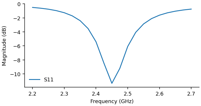
Retrieve the S-parameters from the simulation results and plot the frequency response of the input reflection coefficient ($S_{11}$).

Use sol.s_parameters() to obtain the S-parameter data and plot() to display the frequency response.

freq = sol.frequency
sparam = sol.s_parameters()
sparam.plot()

Reference

[1] The Institute of Electronics, Information and Communication Engineers (IEICE), Technical Committee on Electronics Simulation Technology, “Rectangular Patch Antenna (Probe-Fed),” Canonical Problems for Electromagnetic Simulators.

[2] Takuichi Hirano, Hiroshi Okabe, and Shinichiro Ohnuki, “Canonical Problems for Electromagnetic Simulators — Excitation Modeling with Connectors,” Microwave Workshops & Exhibition (MWE 2014), Workshop 07, December 11, 2014.